2 Overview of scRNA-seq processing pipeline

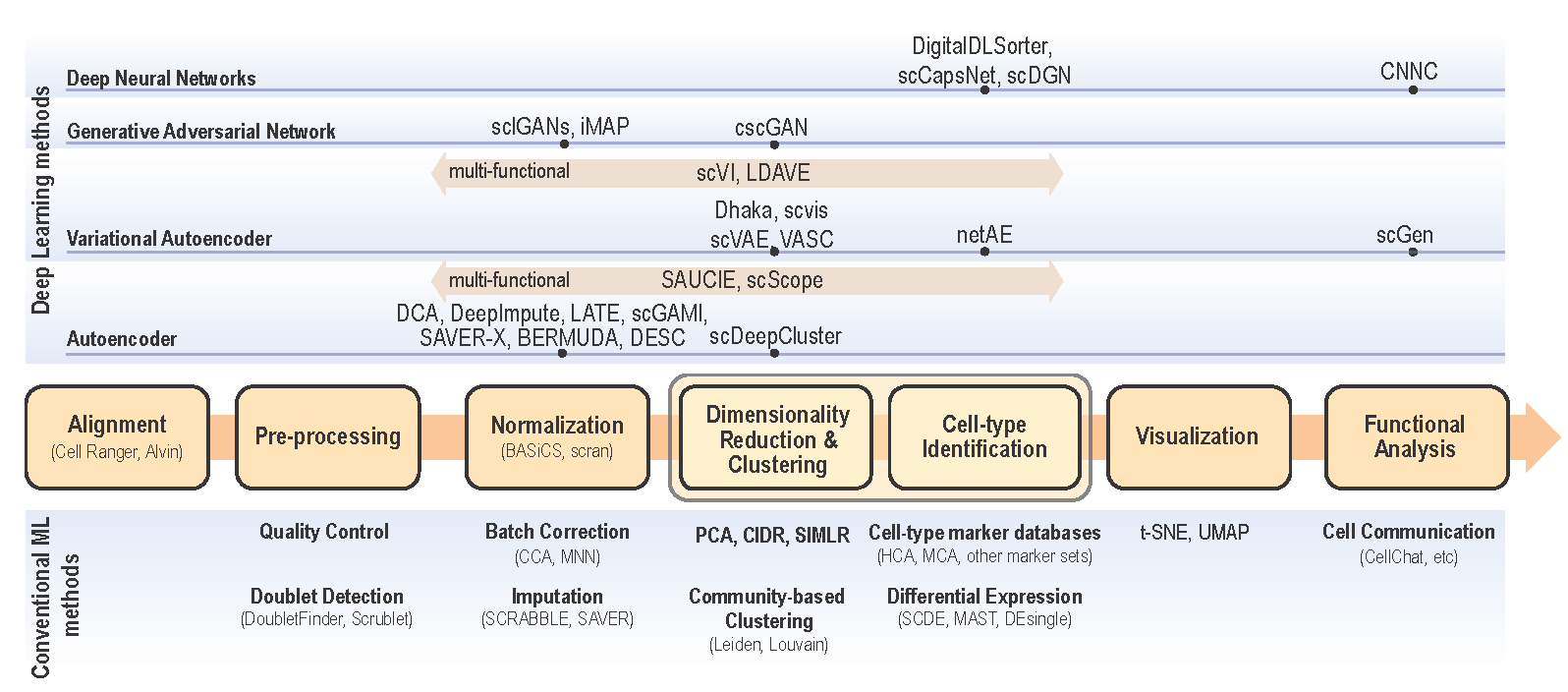
Various scRNA-seq techniques (like SMART-seq, Drop-seq, and 10X genomics sequencing (Eisenstein 2020; Vallejos, Marioni, and Richardson 2015) are available nowadays with their sets of advantages and disadvantages. Despite the differences in the scRNA-seq techniques, the data content and processing steps of scRNA-seq data are quite standard and conventional. A typical scRNA-seq dataset consists of three files: genes quantified (gene IDs), cells quantified (cellular barcode), and a count matrix (number of cells x number of genes), irrespective of the technology or pipeline used. A series of essential steps in scRNA-seq data processing pipeline and optional tools for each step with both ML and DL approaches are illustrated in Fig.2.1.

Figure 2.1: Single cell data analysis steps for both conventional ML methods (bottom) and DL methods (top). Depending on the input data and analysis objectives, major scRNA-se analysis steps are illustrated in the center flow chart. The convential ML approaches along with optional analysis modules are presented below each analysis step. Deep learning approaches are categorized as neural network models (DNN, CNN, CapsNet, and DANN), Generalive Adversarial Network (GAN), Variational Autoencoder, and Autoencoder. For each DL approach, optional algorithms are listed on top of each step in the pipeline.

With the advantage of identifying each cell and unique molecular identifiers (UMIs) for expressions of each gene in a single cell, scRNA-seq data are embedded with increased technical noise and biases (Chen, Ning, and Shi 2019).

Quality control (QC) is the first and the key step to filter out dead cells, double-cells, or cells with failed chemistry or other technical artifacts. The most commonly adopted three QC covariates include the number of counts (count depth) per barcode identifying each cell, the number of genes per barcode, and the fraction of counts from mitochondrial genes per barcode (Eisenstein 2020).

Normalization is designed to eliminate imbalanced sampling, cell differentiation, viability, and many other factors. Approaches tailored for scRNA-seq have been developed including the Bayesian-based method coupled with spike-in, or BASiCS (Vallejos, Marioni, and Richardson 2015), deconvolution approach, scran (Lun, Bach, and Marioni 2016), and sctransfrom in Seurat where regularized Negative Binomial regression was proposed (Hafemeister and Satija 2019). Two important steps, batch correction and imputation, will be carried out if required by the analysis:

• Batch Correction is a common source of technical variation in high-throughput sequencing experiments due to variant experimental conditions such as technicians and experimental time, imposing a major challenge in scRNA-seq data analysis. Batch effect correction algorithms include detection of mutual nearest neighbors (MNNs) (Haghverdi et al. 2018) , canonical correlation analysis (CCA) with Seurat (Butler et al. 2018), and Hormony algorithm through cell-type representation (Korsunsky et al. 2019).

• Imputation step is necessary to handle high sparsity data matrix, due to missing value or dropout in scRNA-seq data analysis. Several tools have been developed to “impute” zero values in scRNA-seq data, such as SCRABBLE (T. Peng et al. 2019), SAVER (Huang et al. 2018) and scImpute (W. V. Li and Li 2018). Dimensionality reduction and visualization are essential steps to represent biological meaningful variation and high dimensionality with significantly reduced computational cost. Dimensionality reduction methods, such as PCA, are widely used in scRNA-seq data analysis to achieve that purpose. More advanced nonlinear approaches that preserve the topological structure and avoid overcrowding in lower dimension representation, such as LLE (Roweis and Saul 2000) (used in SLICER (Welch, Hartemink, and Prins 2016)), tSNE (Linderman et al. 2019), and UMAP (Becht et al. 2018) have also been developed and adopted as a standard in single-cell data visualization.

Dimensionality reduction and visualization are essential steps to represent biologically meaningful variations and high dimensionality with significantly reduced computational cost. Dimensionality reduction methods, such as principal component analysis (PCA), are widely used in scRNA-seq data analysis to achieve that purpose. More advanced nonlinear approaches that preserve the topological structure and avoid overcrowding in lower dimension representation, such as LLE (36?) (used in SLICER (Traag, Waltman, and Eck 2019)), tSNE (B. Wang et al. 2017), and UMAP (Finak et al. 2015), have also been developed and adopted as a standard in single-cell data visualization.

Clustering analysis is a key step to identify cell subpopulations or distinct cell types to unravel the extent of heterogeneity and their associated cell-type-specific markers. Unsupervised clustering is frequently used here to categorize cells into clusters by their similarity often taken the aforementioned dimensionality-reduced representations as input, such as community detection algorithm Louvain (Subelj and Bajec 2011) and Leiden (Traag, Waltman, and Eck 2019) , or data-driven dimensionality reduction followed with k-Means cluster by SIMLR (B. Wang et al. 2017) .

Feature selection is another important step in single-cell RNA-seq analysis is to select a subset of genes, or features, for cell-type identification and functional enrichment of each cluster. This step is achieved by differential expression analysis designed for scRNA-seq, such as MAST that used linear model fitting and likelihood ratio testing (Finak et al. 2015); SCDE that adopted a Bayesian approach with a Negative Binomial model for gene expression and Poisson process for dropouts (Kharchenko, Silberstein, and Scadden 2014), or DEsingle that utilized a Zero-Inflated Negative Binomial model to estimate the dropouts (Miao et al. 2018).

Besides these key steps, downstream analysis can include cell type identification, coexpression analysis, prediction of perturbation response, where DL has also been applied. Other advanced analyses including trajectory inference and velocity and pseudotime analysis are not discussed here because most of the approaches on these topics are non-DL based.